Aggregating Data and Thinking in Pictures

Day 2 of the RI workshop, Summer 2023

Austin Cutler

FSU

Class Today

• Going over the HW
• Reinforcing what we’ve learned so far
  • Different types of data
  • Functions used to clean data
  • How we might want to clean data
• Learning more advanced techniques for cleaning data
  • grouping data using group_by()
  • creating summary tables using summarize()
• Toying around with ggplot()

HW Answers

library(tidyverse)

#load in the data
read_csv('class_toy_data.csv') -> data

#this is an easier way to accomplish what we need
#read_csv('class_toy_data.csv', skip = 1) -> data

#using rename instead
## first we remove the unnecessary row and variables
## then we use rename
data %>% 
  slice(-1) %>% 
  select(-c(x1,x11,x12,x13,x14)) %>% 
  rename('age'     = x2,
         'gender'  = x3,
         'educ'    = x4,
         'income'  = x5,
         'app_rat' = x6,
         'pid'     = x7,
         'opp_tex' = x8,
         'gun_opp' = x9,
         'abo_opp' = x10) -> data

# now lets get the data formatted properly
data %>% 
  mutate(age     = parse_number(age),
         income  = parse_number(income),
         app_rat = parse_number(app_rat),
         gun_opp = parse_number(gun_opp),
         abo_opp = parse_number(abo_opp)) -> data

# changing the negative value from approval to NA
data %>% 
  mutate(app_rat = case_when(app_rat < 0 ~ NA_real_,
                             TRUE ~ app_rat)) -> data

# keeping only republicans
data %>% 
  filter(pid == 'Republican') -> data

# saving the data
#write_csv(data, 'cutler_hw1_data')

# note that this could all technically be done in one big chunk
data %>% 
  slice(-1) %>% 
  select(-c(x1,x11,x12,x13,x14)) %>% 
  rename('age'     = x2,
         'gender'  = x3,
         'educ'    = x4,
         'income'  = x5,
         'app_rat' = x6,
         'pid'     = x7,
         'opp_tex' = x8,
         'gun_opp' = x9,
         'abo_opp' = x10) %>% 
  mutate(age     = parse_number(age),
         income  = parse_number(income),
         app_rat = parse_number(app_rat),
         gun_opp = parse_number(gun_opp),
         abo_opp = parse_number(abo_opp),
         app_rat = case_when(app_rat < 0 ~ NA_real_,
                             TRUE ~ app_rat)) %>% 
  filter(pid == 'Republican')

#alternative ways to accomplish getting the data in the right format:
read_csv('class_toy_data.csv', skip = 1)

#or if we hadn't done that
data %>% 
  mutate(across(c(age,income,app_rat,gun_opp,abo_opp), ~parse_number(.)))

#or we could even just
data %>% 
  mutate(across(where(is.numeric), parse_number))

Brief review

1. What are the types of data we can encounter?

   Show Answer

   Numeric, string/character, factor, logical

2. What is an object in R and where are they shown?

   Show Answer

   Created data, can be either a vector or data frame; global environment

3. What is this %>% called?

   Show Answer

   A “Pipe”

4. What functions did we learn about last class to clean data?

   Show Answer

   mutate(), select(), slice(), filter(), parse_number()

5. What functions can be used to rename variables?

   Show Answer

   rename(), clean_names()

Cleaning Data (cont.)

• The main movers for cleaning data are mutate(), select(), and filter()
• Functions can be used within other functions, and case_when() is very useful for shaping data when combined with mutate()

Cleaning Data Practice

library(tidyverse)

tibble("Full Name" = c("John Smith", "Jimmy Dean", "Robert Williams", 
                       "Emily Davis", "Michael Brown"),
  "Political Affiliation" = c("Democratic", "Republican", NA, "Democratic",
                              "Libertarian"),
  "Represented State" = c("California", "Texas", "New York", NA, "Florida"),
  "Politician Age" = c(45, 65, 60, 41, 20),
  "Years Served" = c(6, NA, 2, 4, 12),
  "Votes Received" = c(24000, NA, 15000, 20000, 32000),
  "Legislation Passed" = c(12, 10, NA, 6, 15)) -> real_congress

real_congress

# A tibble: 5 × 7
  `Full Name`     `Political Affiliation` `Represented State` `Politician Age`
  <chr>           <chr>                   <chr>                          <dbl>
1 John Smith      Democratic              California                        45
2 Jimmy Dean      Republican              Texas                             65
3 Robert Williams <NA>                    New York                          60
4 Emily Davis     Democratic              <NA>                              41
5 Michael Brown   Libertarian             Florida                           20
# ℹ 3 more variables: `Years Served` <dbl>, `Votes Received` <dbl>,
#   `Legislation Passed` <dbl>

Cleaning Data Practice

real_congress %>% 
  janitor::clean_names() %>% 
  rename('party' = political_affiliation,
         'state' = represented_state,
         'age' = politician_age) %>% 
  filter(!is.na(party)) %>% 
  mutate(age_cat = case_when(age < 30 ~ "<30",
                             (age >= 30 & age < 60) ~ "30-60",
                             age >= 60 ~ "60+")) %>% 
  select(full_name,party,state,age_cat) -> real_congress_2

real_congress_2

# A tibble: 4 × 4
  full_name     party       state      age_cat
  <chr>         <chr>       <chr>      <chr>  
1 John Smith    Democratic  California 30-60  
2 Jimmy Dean    Republican  Texas      60+    
3 Emily Davis   Democratic  <NA>       30-60  
4 Michael Brown Libertarian Florida    <30    

Live Coding

Now that we’ve covered the basics again, let’s go through a problem together, download the Live Coding 1 data on the course materials page

Live Coding

As a group, we are going to:

1. Rename all the variables
2. Make Categorical Variables for age, experience, legislator’s activeness using committee membership and bill sponsorship, and votes (let’s assume each district has 60,000 voters)
3. Remove NAs from any variables where there are NAs
4. Make the data set only have their name, party, and the categorical variables from above

Aggregating Data

• In some applications, it is useful to get aggregate level information about our data
• We can use group_by() and summarize() to accomplish this
• group_by works similarly to row_wise() from the homework, let’s start there

Aggregating Data

real_congress %>% 
  janitor::clean_names() %>% 
  rename('party' = political_affiliation,
         'state' = represented_state,
         'age' = politician_age) %>% 
  filter(!is.na(party)) -> real_congress

real_congress

# A tibble: 4 × 7
  full_name     party state   age years_served votes_received legislation_passed
  <chr>         <chr> <chr> <dbl>        <dbl>          <dbl>              <dbl>
1 John Smith    Demo… Cali…    45            6          24000                 12
2 Jimmy Dean    Repu… Texas    65           NA             NA                 10
3 Emily Davis   Demo… <NA>     41            4          20000                  6
4 Michael Brown Libe… Flor…    20           12          32000                 15

• What are some ways we’d be interested in grouping this data?

Aggregating Data

• Finding group numbers

real_congress %>% 
  group_by(party) %>% 
  summarize(sample = n())

# A tibble: 3 × 2
  party       sample
  <chr>        <int>
1 Democratic       2
2 Libertarian      1
3 Republican       1

• What do you notice about the data produced here?

Aggregating Data

real_congress %>% 
  mutate(age_cat = case_when(age < 30 ~ "<30",
                             (age >= 30 & age < 60) ~ "30-60",
                             age >= 60 ~ "60+")) %>% 
  group_by(age_cat) %>% 
  summarize(n())

# A tibble: 3 × 2
  age_cat `n()`
  <chr>   <int>
1 30-60       2
2 60+         1
3 <30         1

Aggregating Data

• We can also use this same style of coding to apply functions to categorical groups

real_congress %>% 
  group_by(party) %>% 
  summarize(age = mean(age))

# A tibble: 3 × 2
  party         age
  <chr>       <dbl>
1 Democratic     43
2 Libertarian    20
3 Republican     65

Aggregating Data

real_congress %>% 
    mutate(age_cat = case_when(age < 30 ~ "<30",
                             (age >= 30 & age < 60) ~ "30-60",
                             age >= 60 ~ "60+")) %>% 
  group_by(age_cat) %>% 
  summarize(leg_pro = mean(legislation_passed))

# A tibble: 3 × 2
  age_cat leg_pro
  <chr>     <dbl>
1 30-60         9
2 60+          10
3 <30          15

• Notice how the data is ordered in a weird way, how could we fix that?

Show Answer

Change the variable from character to factor

Aggregating Data

real_congress %>% 
    mutate(age_cat = case_when(age < 30 ~ "<30",
                             (age >= 30 & age < 60) ~ "30-60",
                             age >= 60 ~ "60+"),
           age_cat = factor(age_cat,
                            levels = c('<30', '30-60', '60+'))) %>% 
  group_by(age_cat) %>% 
  summarize(leg_pro = mean(legislation_passed))

# A tibble: 3 × 2
  age_cat leg_pro
  <fct>     <dbl>
1 <30          15
2 30-60         9
3 60+          10

• Note that the order matters! If we try reversing this, the code won’t work

Aggregating Data

real_congress %>% 
    mutate(age_cat = factor(age_cat,
                            levels = c('<30', '30-60', '60+')),
           age_cat = case_when(age < 30 ~ "<30",
                             (age >= 30 & age < 60) ~ "30-60",
                             age >= 60 ~ "60+")) %>% 
  group_by(age_cat) %>% 
  summarize(leg_pro = mean(legislation_passed))

Error in `mutate()`:
ℹ In argument: `age_cat = factor(age_cat, levels = c("<30", "30-60",
  "60+"))`.
Caused by error in `factor()`:
! object 'age_cat' not found

• That is because the code is sequential, and the age_cat variable isn’t in our data until we make it

Live Coding 2

Let’s use these new tools together

Live Coding 2

Together, let’s keep working on that original data and do the following:

1. Change the data so that we have all the original variables, as well as the new categorical variables we made

2. Find the number of “Congress members” who are in each party, as well as 2 of our created categorical variables

3. Find the average age for each party as well as 2 different categorical variables than the previous step

Probably a break here (?)

ggplot

• Now that we’ve all mastered manipulating data, let’s learn how to paint a picture
• R has a default plot function plot() that you should play around with at some point
• Within the tidyverse package, there is a function & package called ggplot
• ggplot is an incredibly powerful method for creating graphics
  • The resources page on the website points out a few books that help learn more on ggplot, for now, lets get into the basics

The Parts of ggplot

• ggplot has several important components
• ggplot() is how any graph is started, it takes the argument of data, and aes() or aesthetic
  • Within aes(), you set things such as the x and y variables
• Rather than using %>% to pipe between lines, we use a +
  • The packages were made by the same guy, I don’t know why he did this but apparently to fix it would be a huge pain in the butt
• “geoms” are how you actually decide what type of graph you’re making
  • Some examples are geom_bar(), geom_density(), or geom_point()
• Lastly, the theme, which determines how the graph is presented
  • You can use preset option, such as theme_minimal() or theme_classic() or use the theme() function to change things individually, or both together!

Structure of ggplot Code

• Below is the general structure of ggplot code

ggplot(data, aes(x = x_var,y = y_var))+
  geom_line()+
  theme_minimal()+
  theme(plot.title = element_text(hjust=.5))

• Note the + sign and the different sections of the code
• The second line specifies that we are making a line graph
• We can also combine what we’ve learned so far with this structure like so

data %>% 
  mutate(new_var = case_when(x_var = ...)) %>% 
  ggplot(aes(x = new_var, y = y_var))+
    geom_line()+
    theme_minimal()+
    theme(plot.title = element_text(hjust=.5))

Structure of ggplot Code

• There are many ways to graph an average using ggplot, for now, we can use the code from above on finding a group average and go from there

real_congress %>% 
  group_by(party) %>% 
  summarize(age_av = mean(age)) %>% 
  ggplot(aes(x = party, y = age_av))+
  geom_bar(stat = 'identity')+
  theme_minimal()

• Note that within geom_bar() we had to set stat to “identity”

Stucture of ggplot Code

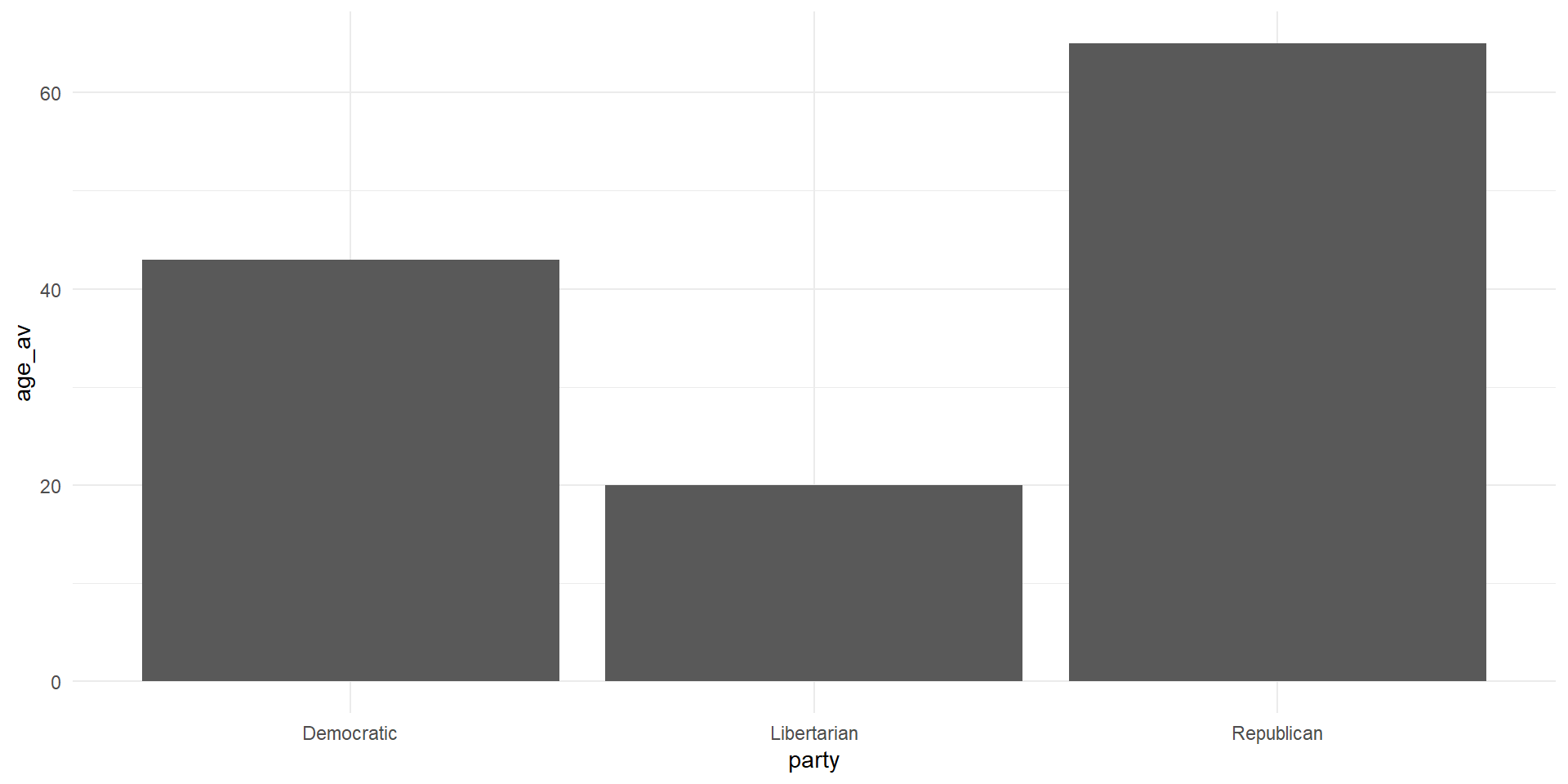
What’re some ways we can make this figure more appealing?

Ways to Improve the Figure

1. Change the axis labels to something that makes sense
2. Add color to each bar
3. Maybe we want a title?
4. A caption of where the data is from?

There are more options, these ideas are meant to get you thinking. A figure is meant to communicate data effectively.

Live Coding 3

Let’s make a pretty picture

Live Coding 3

This section will be a little different. Now that we’re fairly familiar with this data, lets think of some interesting figures we could make!