library(tidyverse)
library(janitor)

#pulling the data set and putting it into R
startdata <- read.csv('CES.csv')

#renaming the data and specific variables, many were already
# a good name
renameddata <- startdata %>%
  rename(gender = gender4,
         mediause = CC22_300_1,
         mentalhealth = CC22_309f,
         generalhealth = CC22_309e,
         presvote20 = presvote20post,
         ideo_self = ideo5)
# other variables that did not need to be renamed: race, pid3,
#pid7, newsint, birthyr

#grabbing only the variables I am interested in
selecteddata <- renameddata %>%
  select(gender, race, pid3, pid7, mediause, mentalhealth, generalhealth,
         presvote20, ideo_self, newsint, birthyr)

#removing any NAs in data
selecteddata %>%
  filter(!is.na(gender),
         !is.na(race),
         !is.na(pid3),
         !is.na(mediause),
         !is.na(mentalhealth),
         !is.na(generalhealth),
         !is.na(presvote20),
         !is.na(ideo_self),
         !is.na(newsint),
         !is.na(pid7),
!is.na(birthyr))Factor variables and Thinking in Pictures
Day 3 of the RI workshop, Summer 2024
Actually Using ggplot Code
- There are many ways to graph an average using ggplot, for now, we can use the code from above on finding a group average and go from there
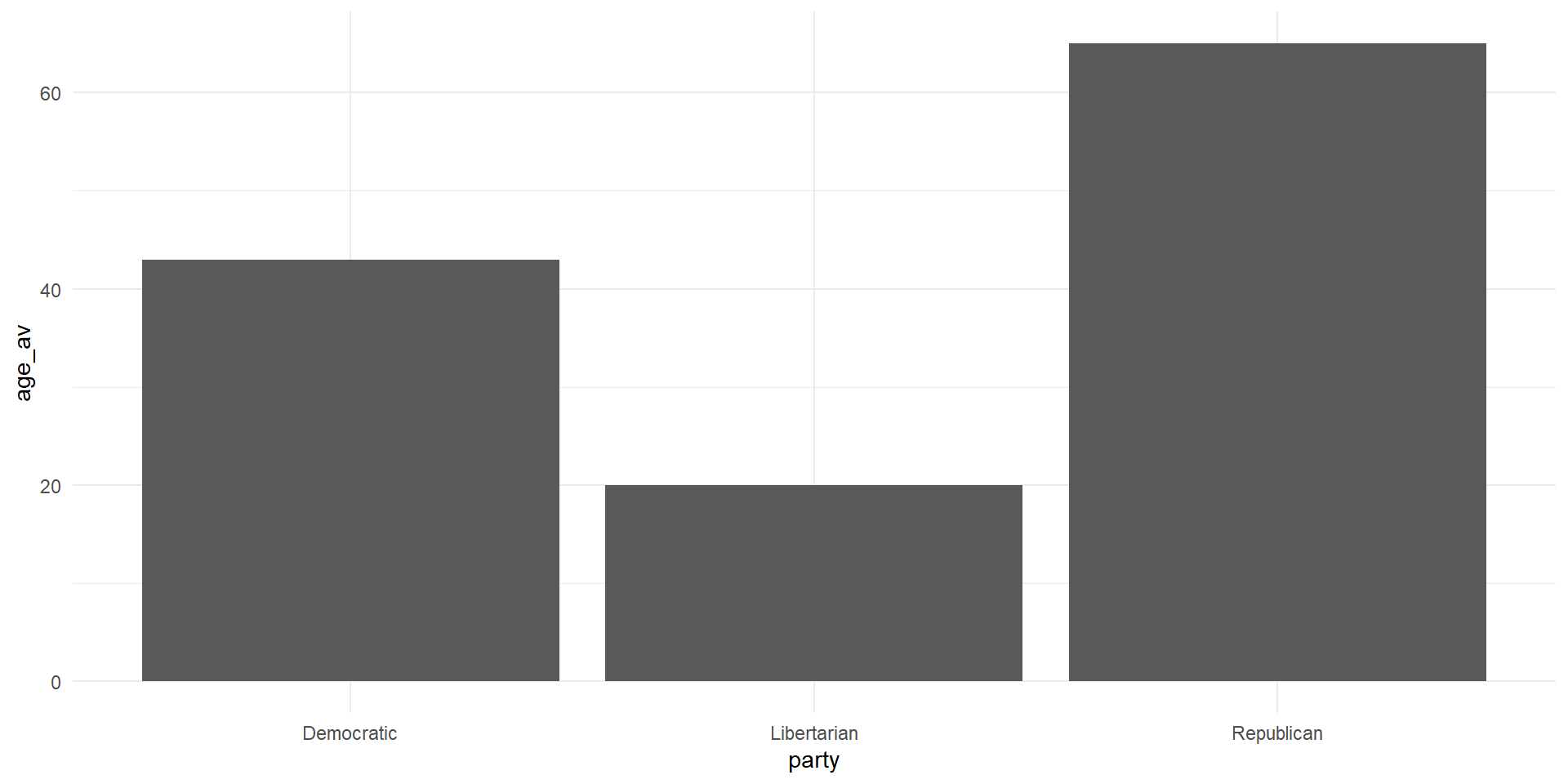
- Note that within
geom_bar()we had to setstatto “identity”
A Graph

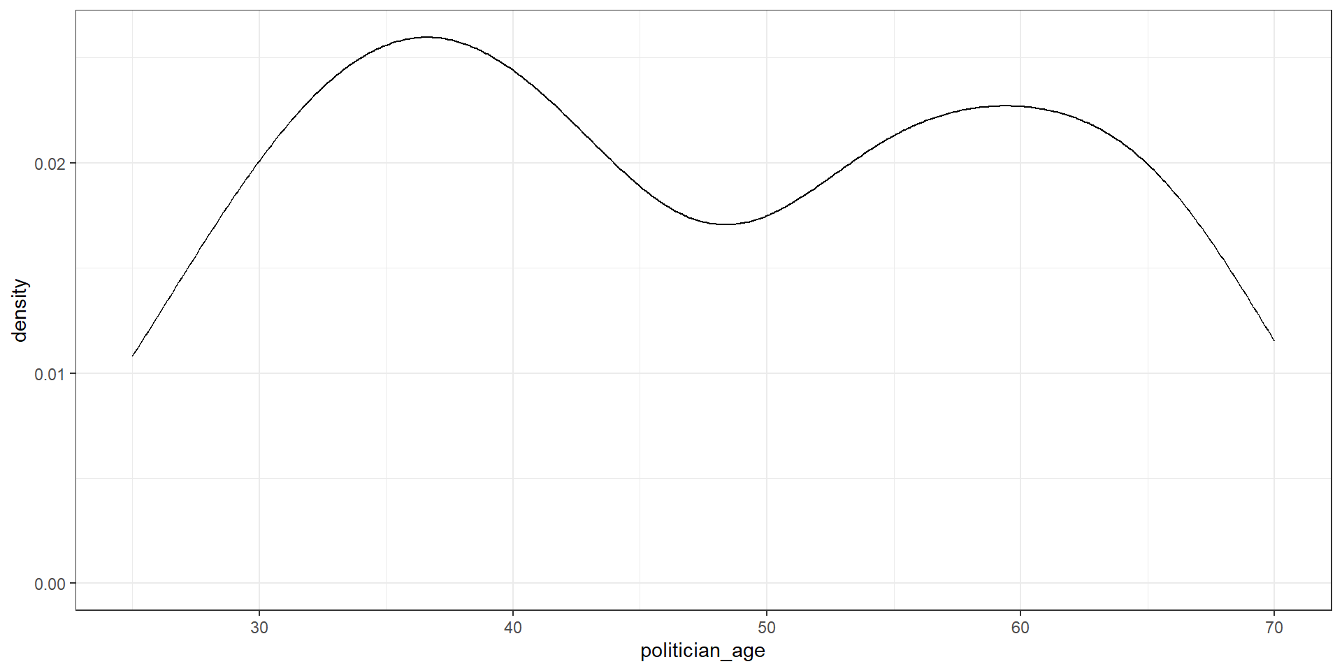
A Density Plot
Another Bar Graph
cong_data %>%
  mutate(party = factor(political_affiliation,
                        levels = c('Democratic',
                                   'Independent',
                                   'Republican',
                                   'Libertarian'))) %>%
  group_by(party) %>%
  summarize(avg = mean(legislation_passed)) %>%
  ggplot(aes(x = party, y = avg))+
  geom_bar(stat = 'identity')+
  labs(x = 'Party', y = 'Average Legislation Passed')+
  theme_classic()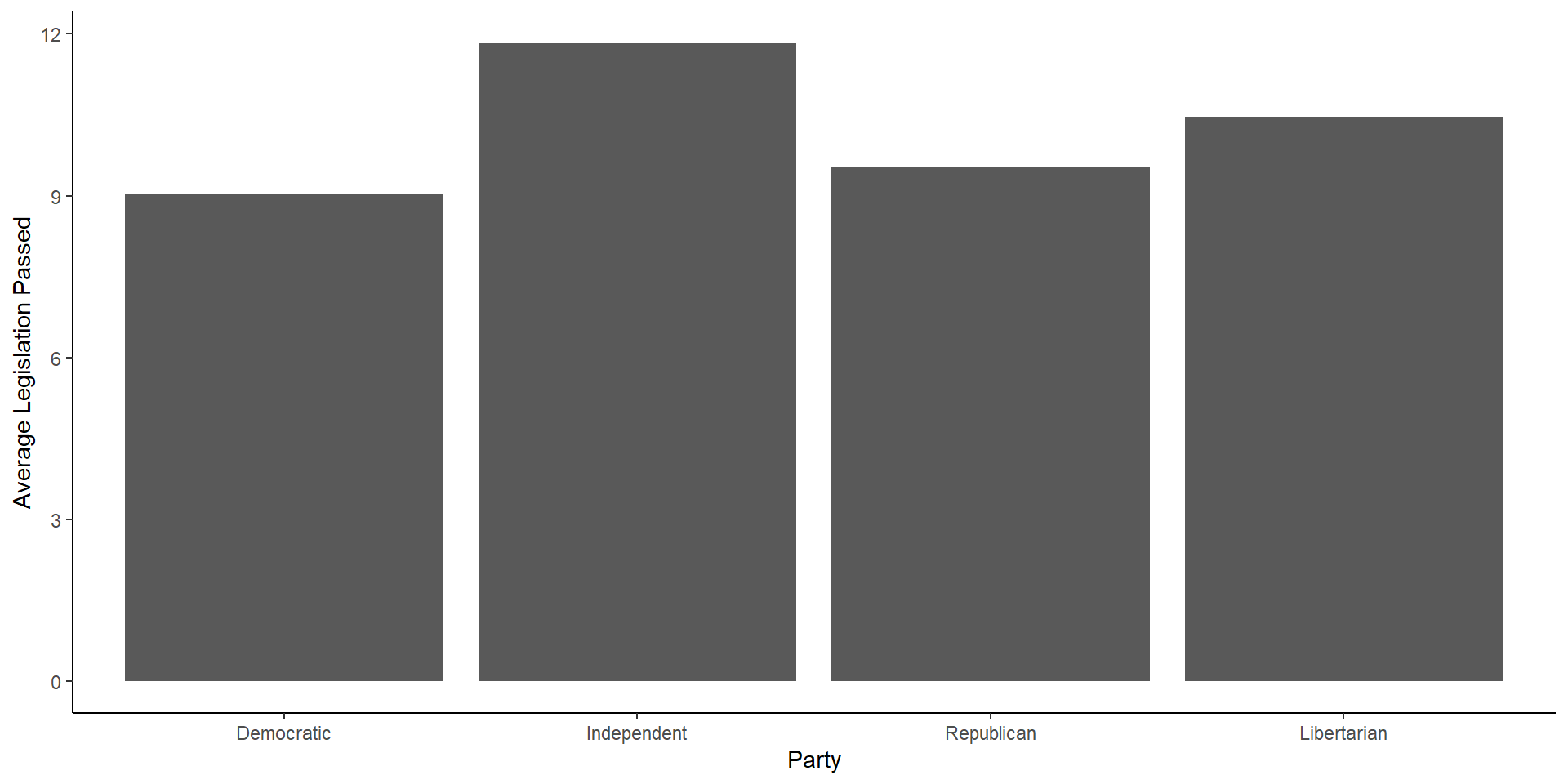
Another Bar Graph

A Touch of Color
cong_data %>%
  mutate(party = factor(political_affiliation,
                        levels = c('Democratic',
                                   'Independent',
                                   'Republican',
                                   'Libertarian'))) %>%
  group_by(party) %>%
  summarize(avg = mean(legislation_passed)) %>%
  ggplot(aes(x = party, y = avg, fill = party))+
  geom_bar(stat = 'identity')+
  labs(x = 'Party', y = 'Average Legislation Passed')+
  theme_classic()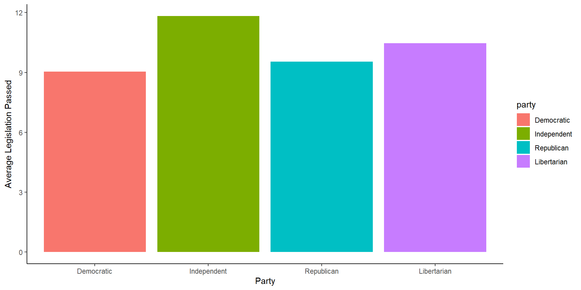
A Touch of Color

Removing the Legend
cong_data %>%
  mutate(party = factor(political_affiliation,
                        levels = c('Democratic',
                                   'Independent',
                                   'Republican',
                                   'Libertarian'))) %>%
  group_by(party) %>%
  summarize(avg = mean(legislation_passed)) %>%
  ggplot(aes(x = party, y = avg, fill = party))+
  geom_bar(stat = 'identity')+
  labs(x = 'Party', y = 'Average Legislation Passed')+
  theme_classic()+
  theme(legend.position = 'none')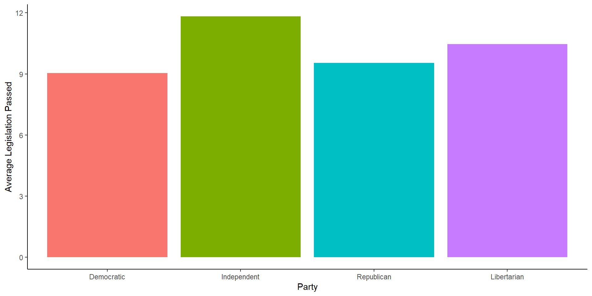
Removing the Legend

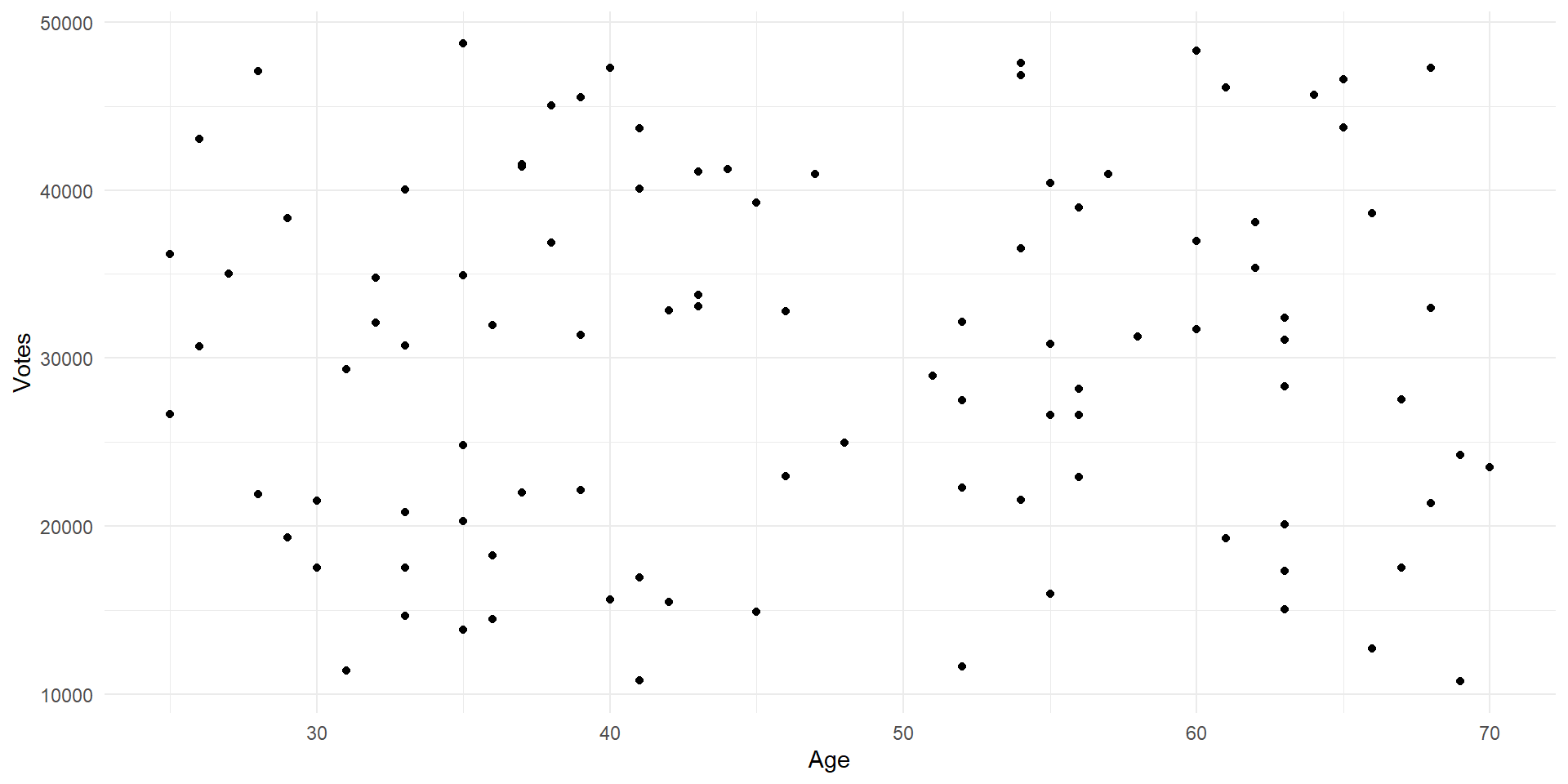
Scatter Plots
- Scatter plots are useful if we have two continuous variables and we want to show their relationship
- We can also make line graphs, but scatter plots show us what the observations look like as well as the general relationship

Scatter Plots
Scatter Plot Size
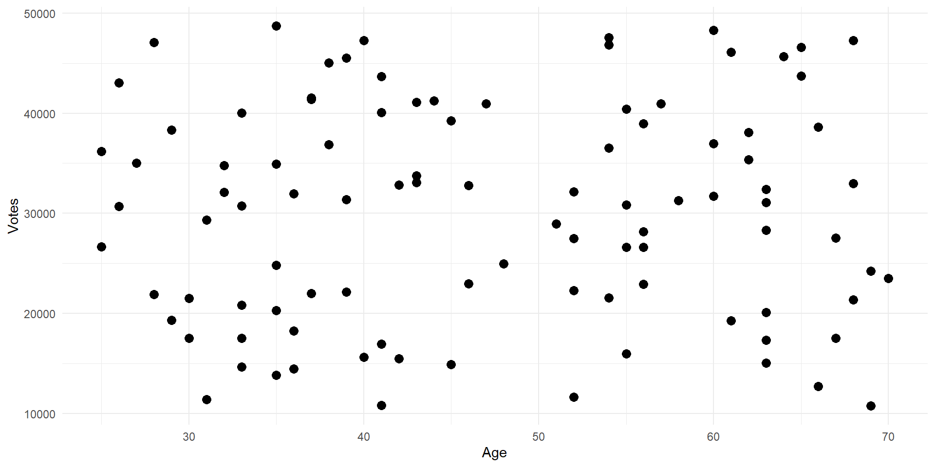
Scatter Plot Size
