R2 Day 2

More loops, simulating data, and plots

Austin Cutler

FSU

Agenda

In today’s class, we’re going to go over the following:
- More practice with for loops
- Bootstrap practice
- Practice simulating data
- Confidence intervals with simulations

More Loops

Let’s start with practicing nested for loops
Individually, create a nested loop structure that prints the sixteen weeks of the semester (i.e., Week 1, Week 2, etc.) in an outer loop and then also prints the five work days (i.e., Monday, Tuesday, etc.) in an inner loop.
If you finish this before the others, add in a third loop that prints out the semester as well (i.e., fall, spring)
- Ignore summer and winter for this, since they don’t follow the standard sixteen week structure

But wait, there’s more (loops)

Nested for loops can also be used to fill out the cells in a matrix
This method is very useful for conducting power analysis when you’re testing multiple treatment effect sizes and sample sizes
To do this, you need to apply what we learned in the previous lecture to fill in each element of a matrix

Matrix and Loops Practice

Individually, create a nested loop that creates a matrix containing a multiplication table that goes up to and includes 12x12
In pairs, create two 6x6 matrices, then using a nested loop, perform matrix addition, storing the results as a new 6x6 matrix
- Ensure that the appropriate cells for each matrix are added together

The Bootstrap

The bootstrap is a very nice way of estimating confidence intervals for any quantity of interest
How this approach works is we sample our data with replacement, generating a new dataset with the same number of observations, but some of them are missing, some are repeated, and some only appear once
We then reestimate our quantity of interest, and then we repeat this process 1000-10000 times
This is distinct from using data simulations for estimating confidence intervals
- As we’ll discuss later, when we simulate data we will assume a certain distribution for the data
- With this approach, we make no assumptions about the distribution of the underlying data generating process

The Bootstrap (in Code)

The functions you’ll want to be most familiar with are sample() and slice_sample()
sample() will take a sample from a vector, and slice_sample() will take a sample from a data frame
In sample() the argument to decide how large of a sample you’ll take is size, and for slice_sample(), it is n
In both cases, we’ll want to set this equal to the size of our original data, and set the argument replace to be TRUE

The Bootstrap (in Code)

Here’s an example of the bootstrap for the mean:

n_sim <- 1000

results <- c()

for(i in 1:n_sim){
  set <- slice_sample(data, n = nrow(data), replace = TRUE)
  
  mean(set$var) -> results[i]
}

ci <- quantile(results, probs = c(.025, .975))

Pull yourself up by…

Using the USJudgeRatings, first estimate the minimum, mean, and maximum of each variable
- You can do this either using a for loop or by using the summarize() function from tidyverse
For each of these quantities, estimate confidence 95% confidence intervals using the bootstrap
Get standard 95% confidence intervals for the mean and compare them to the bootstrap confidence intervals

Simulations

Simulating Data

In doing quantitative social science, simulating data is a very important tool in your toolkit
- Monte Carlo simulations for power
- Conducting analysis on a rare phenomenon
- Estimating confidence intervals (more ways than bootstrapping, see King, Tomz, and Wittenburg (2000))
- Randomization inference and treatment assignment mechanisms
- Creating toy data examples to explore and demonstrate problems, or as a proof of concept
  - Or to teach methods to undergraduates or grad students

Simulating Data

To simulate data, we will most often use the “r” functions from the sets of built in, distribution family functions in r
- rbinom(), rnorm(), rnbinom(), rmvnorm()*, etc.
These functions all have companion functions that give you the pdf of a given distribution for whatever data you put in,
- pbinom(), pnorm(), pnbinom(), pmvnorm()*, etc.
- there are also “d” functions for the density, and “q” functions for the quantiles
- These two functions come from the mvtnorm package, while the rest are in base R

`rbinom()`

One of the most common simulations you’ll do is simulating Bernoulli Trials for random treatment assignment
To do this, we will use rbinom()

#Bernoulli trial for 150 units
b_vec1 <- rbinom(n = 150, size = 1, prob = .5)
head(b_vec1)

[1] 1 1 0 1 0 1

n is the number of observations, size is the number of trials per observation, and prob is the probability of a successful trial
- In practice, you’ll most often be changing n or prob

`rbinom()` practice

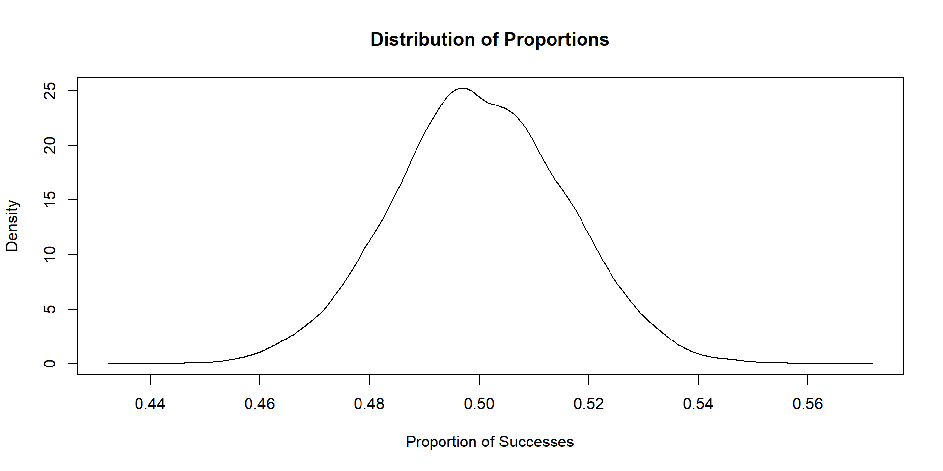
Simulate 10,000 Bernoulli trials
For each trial, set the number of observations to be 1000, with the probability of a “success” being .5
For each trial, estimate the proportion of units that succeed, and store this estimate in a vector
After all 10,000 trials, plot the distribution of that vector (using plot or ggplot)

Plot

Code

n_sim <- 10000
results <- rep(NA, n_sim)

for (i in 1:n_sim) {
  sim <- rbinom(1000, 1, .5)
  
  results[i] <- mean(sim)
}

plot(density(results),main = 'Distribution of Proportions', xlab = 'Proportion of Successes')

Simulating the Normal Distribution

We can also simulate draws from the standard normal distribution
To do this, we use the rnorm() function
The syntax of the code is nearly identical, but instead rnorm() takes the arguments mean and sd

Practice with `rnorm()`

Use a for loop to plot histograms of the standard normal distribution over 3 sample sizes: n = 10, n = 50, and n = 1000
Repeat the previous step, but by varying the mean and standard deviation as well
- Bonus points if you incorporate the paramater value changes in your plot titles
- Reminder: plots can be stored as objects, and saved in lists

Simulating Matrices

We can also us rnorm() to simulate an entire matrix
An example of how we would do this is as follows:

# creating a matrix using the standard normal distribution
mat <- matrix(rnorm(4000), ncol = 4)
head(mat)

           [,1]       [,2]       [,3]       [,4]
[1,]  1.6609885  0.5292288 -0.2973597 -1.0798235
[2,]  0.7807043  1.2587961 -1.3832009 -2.3535789
[3,] -0.5396074  0.6998001  0.9047782 -1.4692511
[4,]  0.2365920 -1.0059394 -0.3580972  0.9208851
[5,]  0.1890745 -0.7260650  0.3786667 -0.6581734
[6,]  0.7461223 -0.7676132  0.9537298 -0.5252005

Simulating Matrices

We can also simulate multiple distributions in a single matrix:

# creating a matrix using the standard normal distribution
mat2 <- matrix(c(rnorm(3000),rbinom(1000,1,.5)), ncol = 4)
head(mat2)

            [,1]       [,2]       [,3] [,4]
[1,]  0.48793932  0.2840526 -0.1178434    0
[2,] -0.72609351  0.8127428  0.3048668    1
[3,]  0.08315486  1.8190829  1.2636292    0
[4,]  0.21056237  0.4234619  0.3069175    0
[5,]  0.04226511 -2.2886926  1.6162669    0
[6,]  0.03433358  0.1398568  0.7513261    0

Uncertainty Estimation with Monte Carlo Simulations

Multivariate Normal Distribution

King, Tomz, and Wittenberg (2000) proposed a new method of estimating uncertainty for regression coefficients using the multivariate normal distribution
The multivariate normal distribution is very similar to the standard normal, however \(\mu\) is now a vector of means, and instead of \(\sigma\), the variance is \(\Sigma\), which is a variance-covariance matrix
To use this method for uncertainty estimation, you:
- Estimate your regression
- Extract the coefficients to be used as \(\mu\)
- Extract your variance-covariance matrix for \(\sigma\)
- Simulate draws from the multivariate normal
- Quantile method

Practice

For this problem, we’re going to use the data under Day 2 on the website
This data consists of the stats and names of each pokemon from generation 1-6, as well as how often they are used in professional tournaments (as a percentage, but numeric, i.e., 1% is 1, not 0.01)
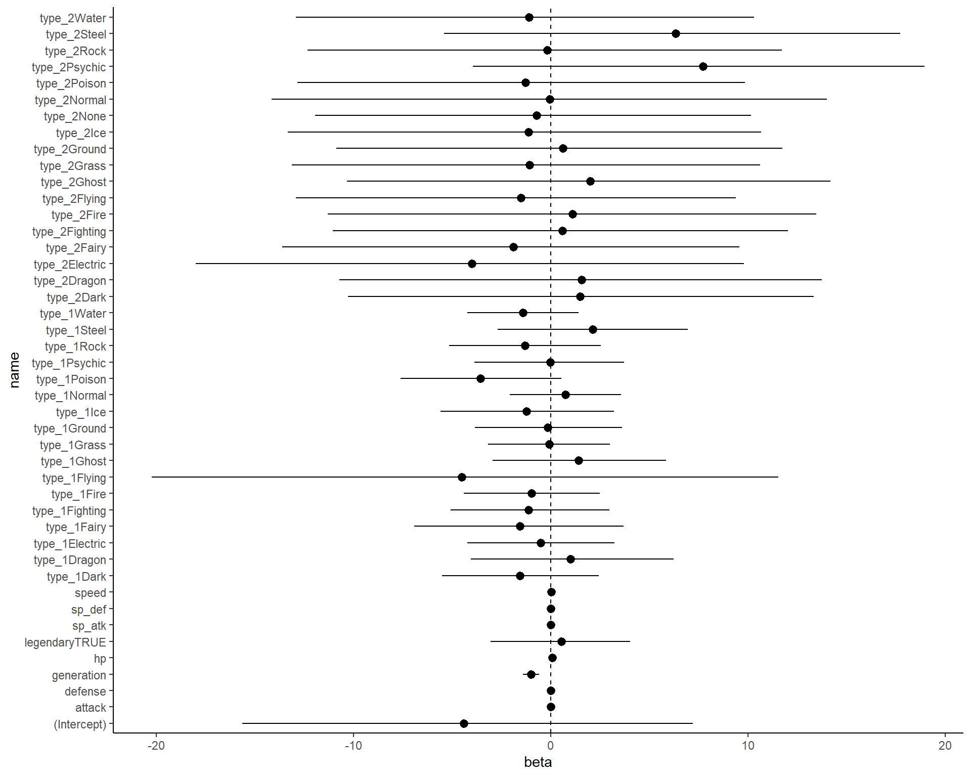
Your goal is to fit a linear regression model to predict tournament usage, then use the KTW method to get 95% confidence intervals.

Practice

First, fit a linear regression model with all covariates (except for total, as you’ll run into multicolinearity issues), regressing pokemon usage onto the remaining covariates
Extract the regression coefficients and variance covariance matrix (the coef() and vcov() functions will help here)
Use the rmvnorm() function from the mvtnorm package to simulate 1000 draws from the multivariate normal, using the coefficients and variance-covariance matrix from step 1
Take the quantiles of each column of the matrix (hint: use the apply function), to get your 95% confidence intervals

Answer

Code

library(tidyverse)

pokemon_data <- read_csv('pokemon_data.csv')

fit <- lm(usage_per ~ type_1+type_2+hp+attack+defense+sp_atk+sp_def+speed+generation+legendary, data = pokemon_data)

as.data.frame(apply(mvtnorm::rmvnorm(10000, mean = coef(fit),sigma = vcov(fit)),
                    2,quantile, probs = c(.025,.975))) %>% 
  pivot_longer(cols = 1:ncol(.)) %>% 
  arrange(name) %>% 
  mutate(qi = rep(c('lower','upper'), time = nrow(.)/2)) %>% 
  pivot_wider(names_from = qi, values_from = value) %>%
  left_join(as.data.frame(coef(fit)) %>% 
              mutate(name = rownames(.))) %>% 
  rename(beta = `coef(fit)`) %>% 
  select(name,beta,lower,upper) %>% 
  ggplot(aes(x = beta, y = name))+
  geom_pointrange(aes(xmin = lower, xmax = upper))+
  geom_vline(aes(xintercept = 0), linetype = 2)+
  theme_classic()

R2 Day 2

Agenda

More Loops

But wait, there’s more (loops)

Matrix and Loops Practice

The Bootstrap

The Bootstrap (in Code)

The Bootstrap (in Code)

Pull yourself up by…

Simulations

Simulating Data

Simulating Data

rbinom()

rbinom() practice

Plot

Simulating the Normal Distribution

Practice with rnorm()

Simulating Matrices

Simulating Matrices

Uncertainty Estimation with Monte Carlo Simulations

Multivariate Normal Distribution

Practice

Practice

Answer

`rbinom()`

`rbinom()` practice

Practice with `rnorm()`