[1] 4Day 3
Let’s get some lunch
Functions to Help with graphs
- Another area where user made functions can be useful is making figures
- Hypothetically, let’s say you were working on a paper for publication and the figures required two distinct aesthetics
Plot
Code
##heteroskedastic
vcov_h <- sandwich::vcovHC(fit)
fit_h <- fit_h <- lmtest::coeftest(fit, vcov = vcov_h)

##clustered-robust
vcov_cr <- sandwich::vcovCL(fit, cluster = data$pid1)
fit_cr <- lmtest::coeftest(fit, vcov = vcov_cr)

##bootstrapped
vcov_bs <- sandwich::vcovBS(fit)
fit_bs <- lmtest::coeftest(fit, vcov = vcov_bs)

##bootstrapped by hand
n_sim <- 10000

coefs  <- list()

for(i in 1:n_sim){
  bs_dat <- slice_sample(data, n = nrow(data), replace = TRUE)

  bs_fit <- lm(out_feel ~ tr, data = bs_dat)

  coefs[[i]] <- tibble(coef = names(coef(bs_fit)),
                       est  = coef(bs_fit))
}

bind_rows(coefs) %>%
  group_by(coef) %>%
  reframe(est = quantile(est, probs = c(.025,.975))) %>%
  mutate(qi = rep(c('lower','upper'),3)) %>%
  pivot_wider(names_from = qi, values_from = est) %>%
  mutate(vcov =  'Bootstrap by Hand') %>%
  left_join(tibble(est  = coef(fit),
                   coef = names(coef(fit)))) -> bs_ci

##making a figure to compare
tibble(est = coef(fit), se = fit_h[,2], vcov = 'Heteroskedastic') %>%
  bind_rows(tibble(est = coef(fit), se = fit_cr[,2], vcov = 'Clustered-Robust'),
            tibble(est = coef(fit), se = lmtest::coeftest(fit)[,2], vcov = 'Standard'),
            tibble(est = coef(fit), se = fit_bs[,2], vcov = 'Bootstrapped')) %>%
  mutate(coef = rep(row.names(fit_h), times = 4),
         lower = est - 1.96*se,
         upper = est + 1.96*se) %>%
  bind_rows(ktw(fit) %>%
              mutate(est =  coef(fit),
                     vcov = 'KTW'),
            bs_ci) %>%
  mutate(vcov  = factor(vcov,
                        levels = c('Standard',
                                   'Heteroskedastic',
                                   'Clustered-Robust',
                                   'Bootstrapped',
                                   'Bootstrap by Hand',
                                   'KTW')),
         coef = str_to_title(str_remove(coef,'tr'))) %>%
  ggplot(aes(x = est, y = fct_rev(coef), color = vcov))+
  geom_pointrange(aes(xmin = lower, xmax = upper),
                   position = position_dodge2(.45,
                                            reverse = TRUE))+
  labs(color = 'Standard Error',
       y = 'Coefficient', x = 'Estimate') +
  scale_color_brewer(palette = 'Set2')+
  theme_b()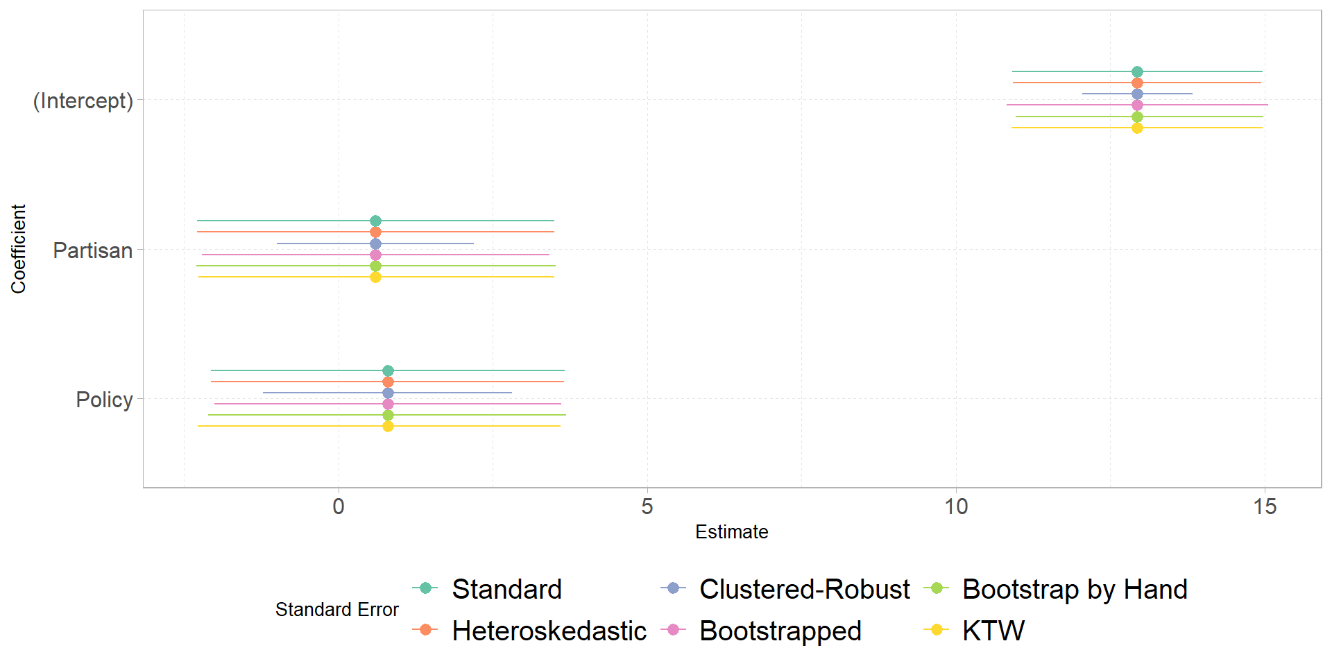
Comments
quartoto produce documents like this, you’ll want to make sure you avoid unnecessary printouts, such as warnings or messages from loaded packages, or just results that do not answer a question (e.g., printing the name of every variable for the dataset used in question 2 when only two of those variables are actually used for the assignment.)#be used for headers, you need a space between the symbol and your titleplot()when you call it