Day 4

Everything Else

Austin Cutler

FSU

Agenda

Final homework check
Optimization
Graphing regression results
Parallelization with map
Advanced Applications of Course Content

Final Homework check in

Let’s get optimal

Optimization

There will be times where you may need to optimize a function in R
When we say optimize, we’re referring to finding the solution to a described problem
- Most often this involves finding a local or global minimum or maximum (i.e., finding the point where our function’s derivative equals 0)
To do this, we can use the optim() function in R

`optim()`

To use optim(), we first need to supply it with a function to optimize (Note: this is another use case for being comfortable with user created functions)
You need to supply optim() with the starting value for the parameters to be optimized over
You also need to define the method being used (we’ll most often use ‘L-BFGS-B’)

`optim()`

Below is an example:

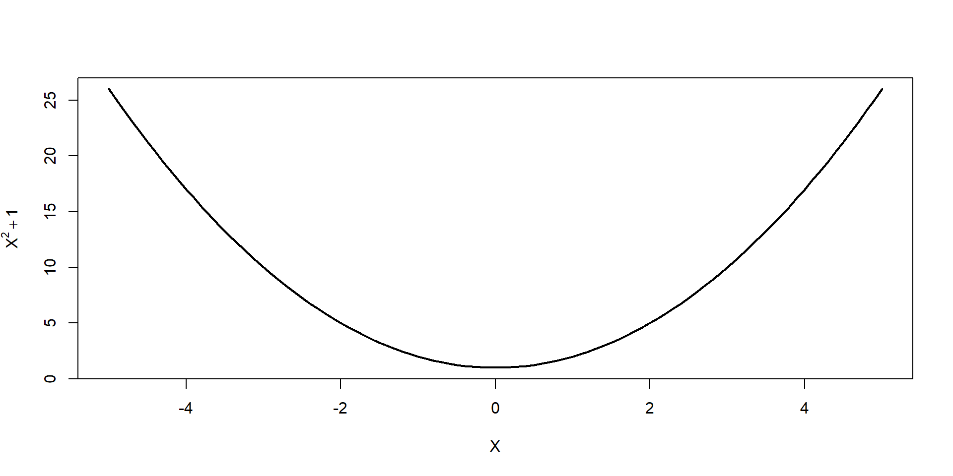
# first I need to define the function I want to optimize
function_1 <- function(x) {
# this function calculates the square of its input and adds 1
x^2 + 1
}
# second, I supply this function to optim()
optim(par = 5, function_1, method = "L-BFGS-B")

$par
[1] 4.984086e-25

$value
[1] 1

$counts
function gradient 
       4        4 

$convergence
[1] 0

$message
[1] "CONVERGENCE: NORM OF PROJECTED GRADIENT <= PGTOL"

`optim()`

The output of optim() is as follows:
- convergence will indicate if the algorithm converged (i.e., if a minimum can be found), will be 0 if it did
- par is the value where the given function is minimized
- value is the global minimum of the function

Maximization

By default, optim() will estimate the minimum, however, we can change this to be the maximum if we add control = list('fnscale' = -1) to our original code

function_2 <- function(x) {
  exp(x)
}

optim(par = 5, function_2, method = "L-BFGS-B",control = list('fnscale' = -1))

Error in optim(par = 5, function_2, method = "L-BFGS-B", control = list(fnscale = -1)): L-BFGS-B needs finite values of 'fn'

Bounded Optimization

In optim(), we can specify lower and upper bounds of the range we want to consider a function, which at times may fix this issue

optim(par = 5, function_2, method = "L-BFGS-B",control = list('fnscale' = -1), lower = -1, upper = 100)

$par
[1] 100

$value
[1] 2.688117e+43

$counts
function gradient 
       2        2 

$convergence
[1] 0

$message
[1] "CONVERGENCE: NORM OF PROJECTED GRADIENT <= PGTOL"

Graphing Functions

Sometimes it is useful to graph functions to better understand how they work
- Or, if you wind up teaching methods, it can be very helpful
To do this with base R, we can use the curve() function
For ggplot, we use the stat_function() function
In both cases, we will need to specify the range of values we want our function graphed over

`curve()`

curve(function_1, from = -5, to = 5, 
      xlab = 'X', ylab = expression(X^2+1), lwd = 2)

`stat_function()`

library(tidyverse)

tibble(x = seq(-5,5,by =  .1)) %>% 
  ggplot(aes(x = x))+
  stat_function(fun = function_1, linewidth = 1)+
  labs(x = 'X', y = expression(X^2+1))+
  theme_classic()

More on Graphing Functions

We can also use optim() to add additional information about the function to our figure
First we need to save the data, then add it to the figures

opt_result <- optim(par = 5, function_1, method = "L-BFGS-B")
# Extract the minimum point
x_min <- opt_result$par
y_min <- opt_result$value

`curve()`

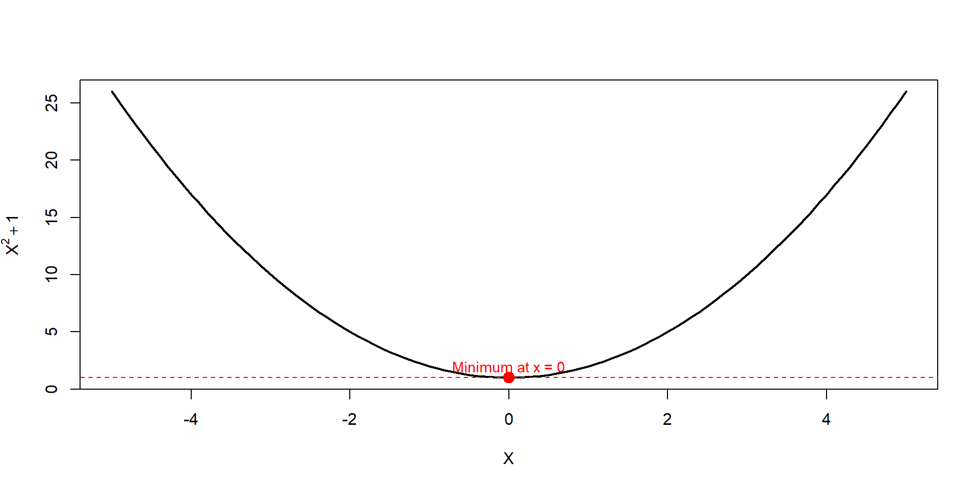
curve(function_1, from = -5, to = 5,
      xlab = 'X', ylab = expression(X^2 + 1), lwd = 2)

# Add red point from optim()
points(x_min, y_min, col = "red", pch = 19, cex = 1.5)

# tangent line
abline(h = y_min, col = "red", lty = 2)

# label
text(x_min, y_min + 1, labels = paste0("Minimum at x = ", round(x_min, 2)), col = "red", cex = 0.9)

`curve()`

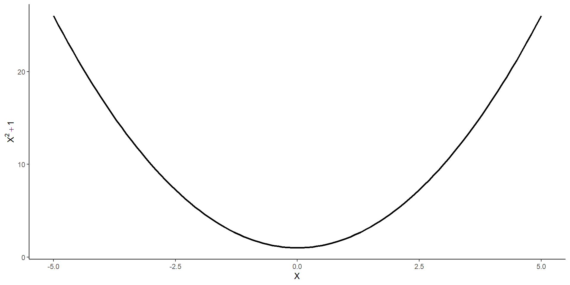
`stat_function()`

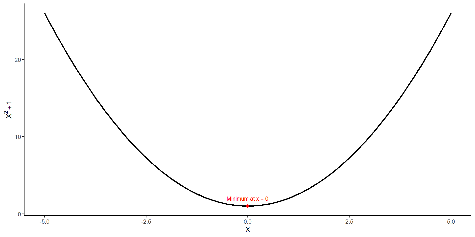
tibble(x = seq(-5, 5, by = 0.1)) %>%
  ggplot(aes(x = x)) +
  stat_function(fun = function_1, linewidth = 1) +
  geom_point(data = tibble(x_min,y_min),
             aes(x = x_min, y = y_min), color = "red", size = 2) +
  geom_hline(yintercept = y_min, linetype = 2, color = "red") +
  annotate("text", x = x_min, y = y_min + 1,
           label = paste0("Minimum at x = ", round(x_min, 2)),
           color = "red", size = 3) +
  labs(x = expression(X), y = expression(X^2 + 1)) +
  theme_classic()

`stat_function()`

Practice

Complete the following problems:

Create a function in R that is a negative quadratic (\(-x^2+10\)). Find the local maximum by hand, and find the maximum using optim(), compare your answers.
Create a function that has a minimum that is not a quadradic. Plot the function, then calculate the value of the function that produces the minimum and maximum using optim().
Create a function that contains both a maximum and a minimum and plot the function. Calculate the value of the function that produces the minimum, the maximum, as well as the values of the minimum and maximum.

Presenting Regression Results

One of the most important skills for being a political scientist is knowing how to present the results of our research
The most important question to ask yourself when presenting results is to ask yourself “what is my quantity of interest?”
The quantity of interest is whatever quantity is being used for the hypothesis test
- The slope of a line
- A difference in means
- The difference between two slopes
- Predicted probabilities across the range of a variable

Coefficient Plots

The most effective way of showing regression results is using a coefficient plot
With the skills you’ve already developed, you can create coefficient plots by hand easily
- This is how I typically will get my results
There are also several packages out there that produce very nice coefficient plots

By Hand

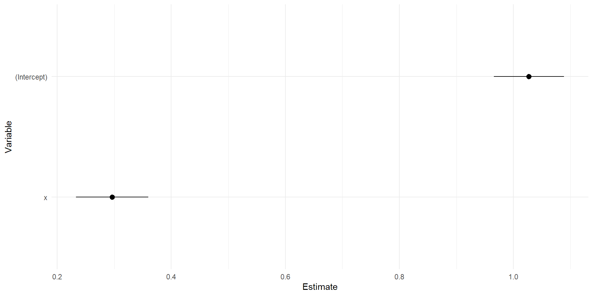
To make a coefficient plot by hand, all you need is your coefficient names, the coefficient value, and the standard error

x  <- rnorm(1000)
y <- 1+.25*x+rnorm(1000)

fit <- lm(y~x)

##extracting standard error
se <-  summary(fit)$coefficients[, "Std. Error"]

#in this case I'm typing the variable names by hand, you can get this out in other ways
tibble(var  = c('(Intercept)','x'),
       coef = coef(fit),
       se   = se) %>% 
  mutate(lower = coef - 1.96*se,
         upper = coef + 1.96*se) -> coef_dat

By Hand

coef_dat %>% 
  ggplot(aes(x = coef, y = fct_rev(var)))+
  geom_pointrange(aes(xmin = lower, xmax = upper))+
  labs(x = 'Estimate', y = 'Variable')+
  theme_minimal()

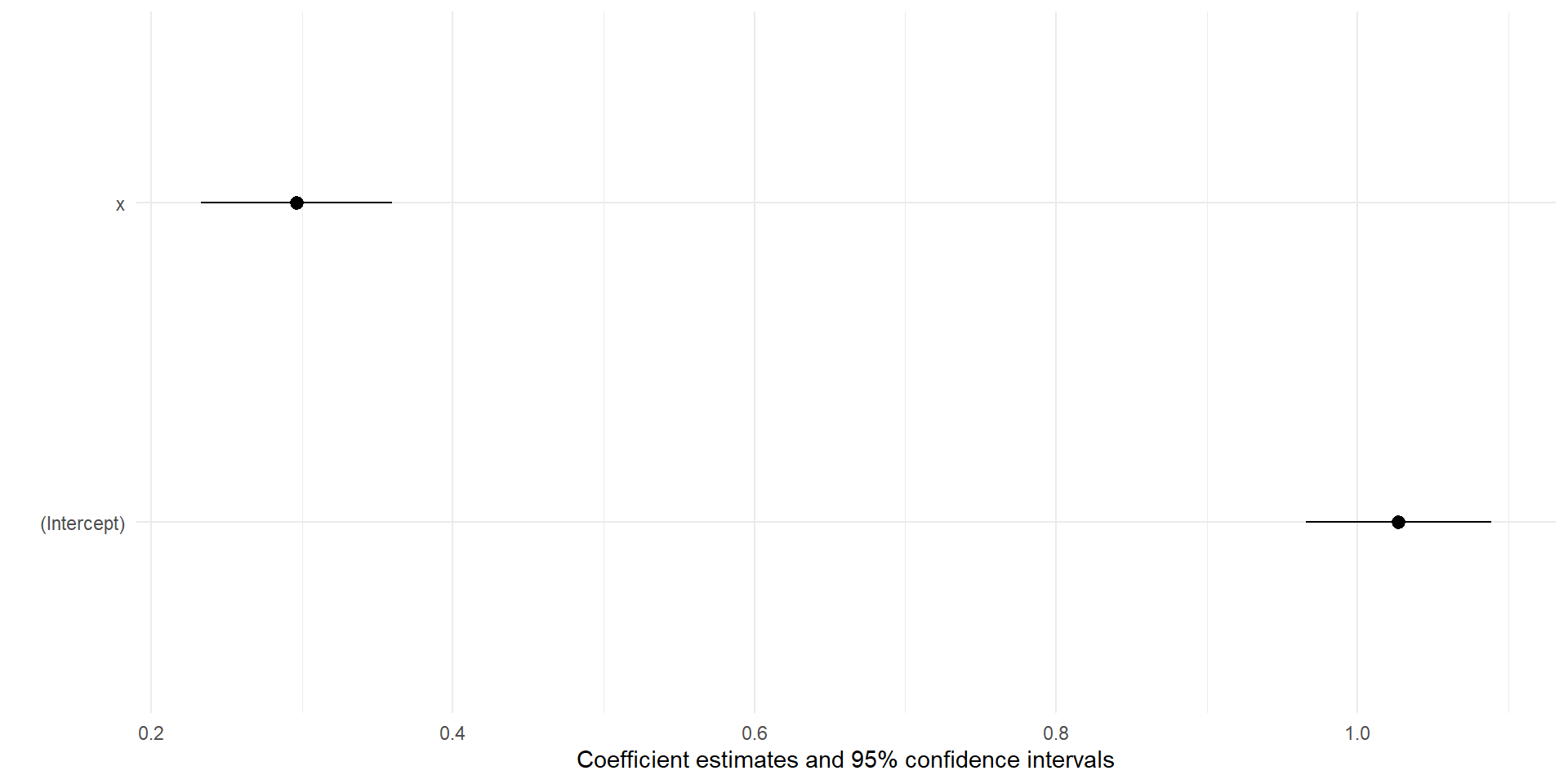
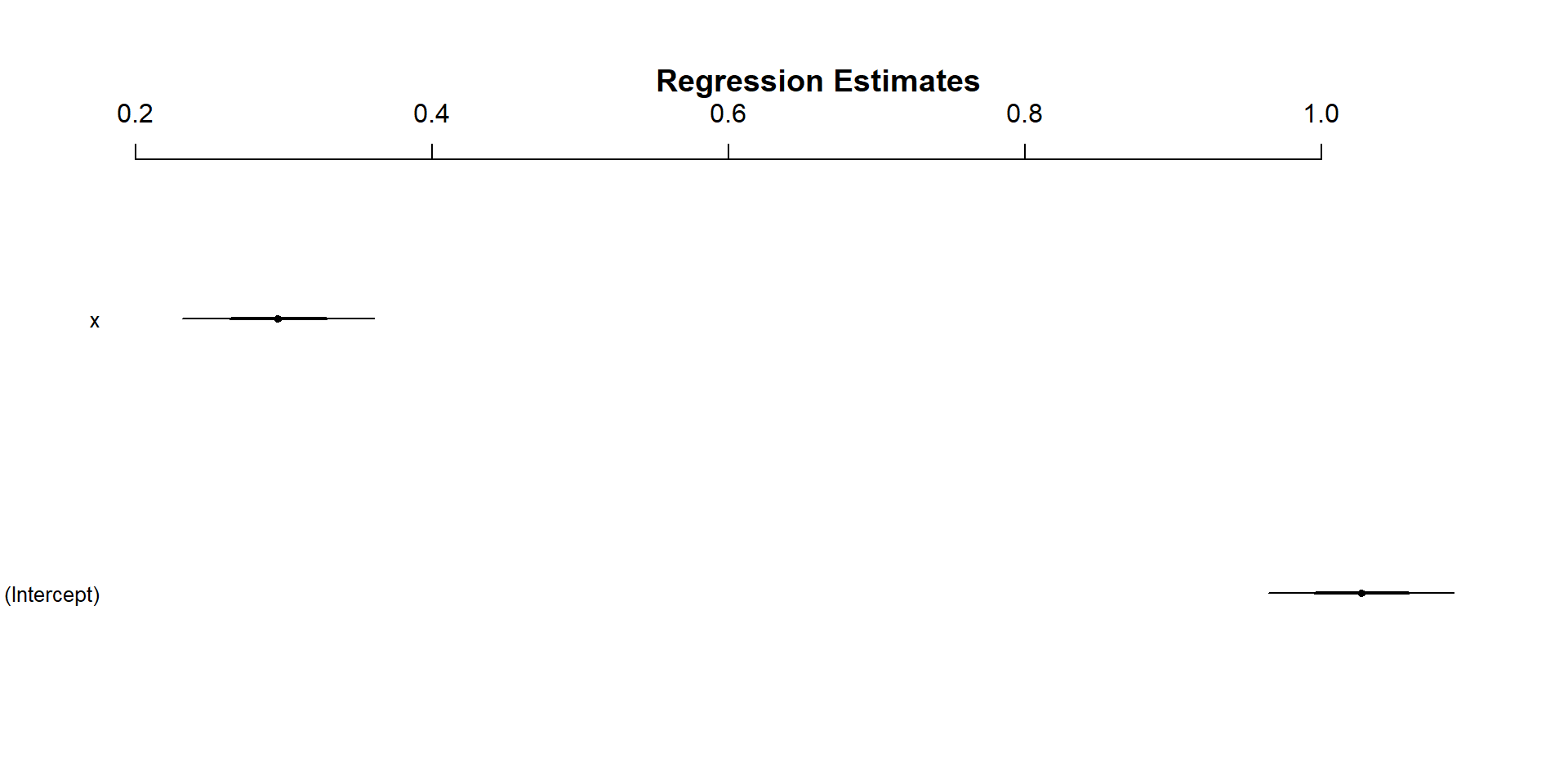
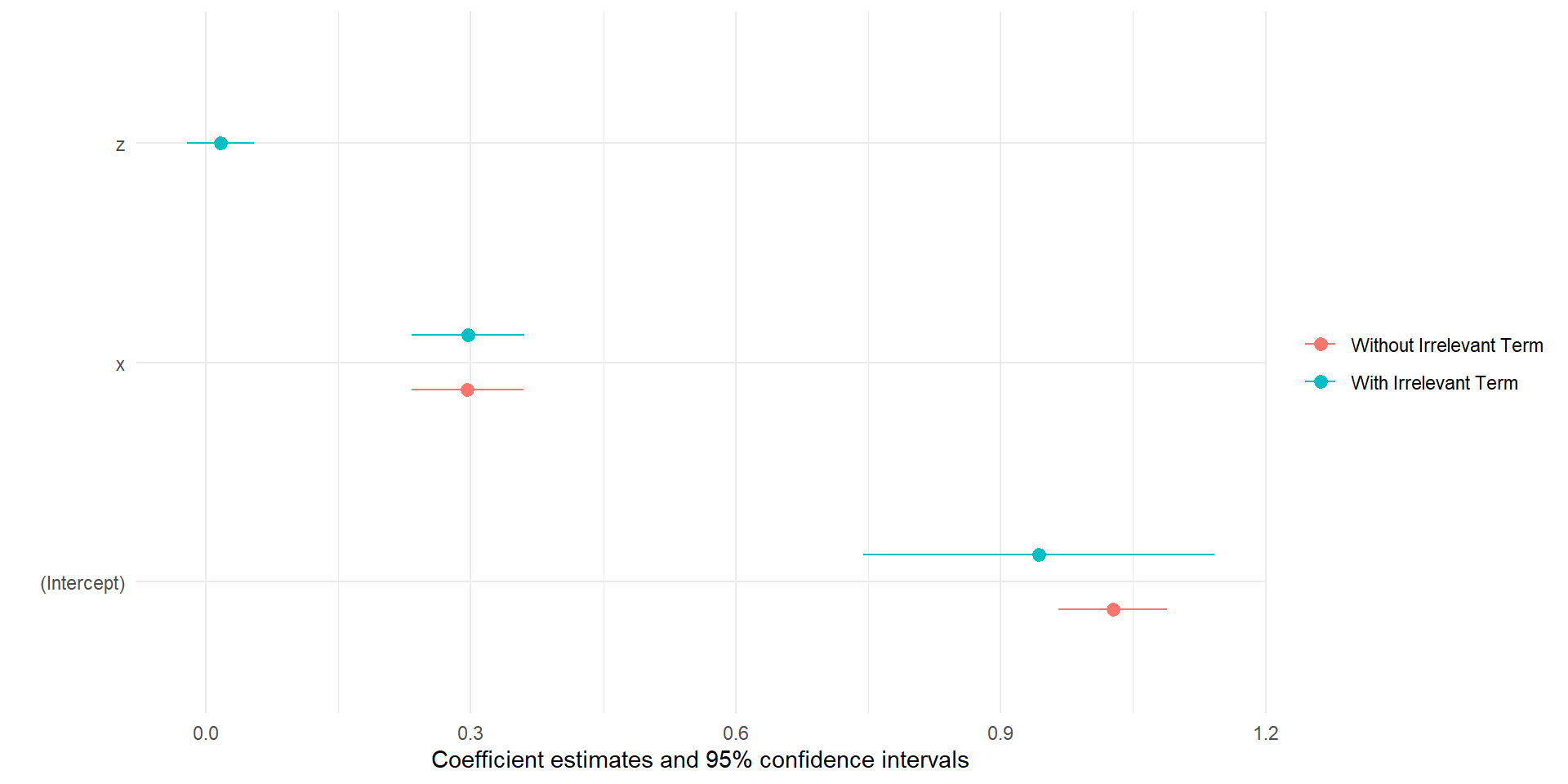
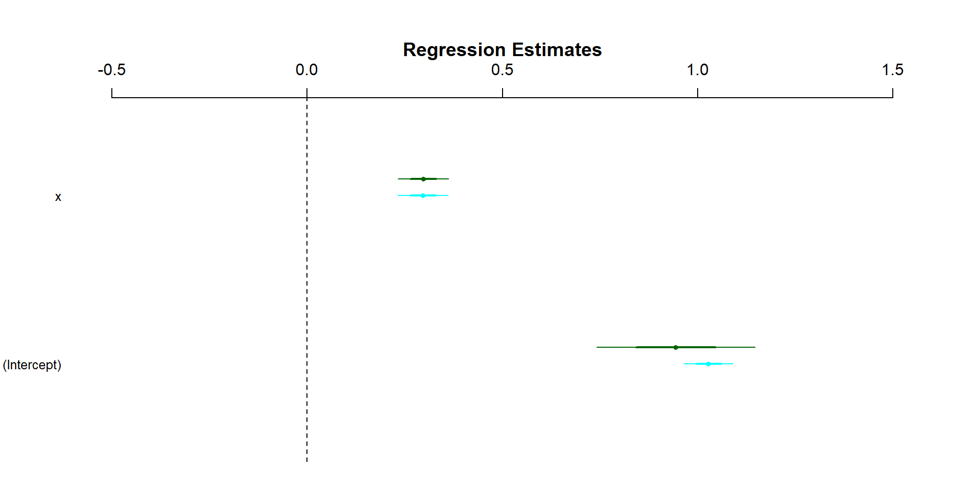
arm, broom, and modelsummary

Broom, arm, and modelsummary are all packages offer caned alternatives to creating the figure by hand
the modelplot() function is from the model summary package

library(broom)
library(modelsummary)
library(arm)

modelplot(fit)

modelsummary

arm

coefplot() is from the arm package

coefplot(fit, intercept = TRUE)

broom

While broom doesn’t have a built in plot function, it is a great way to clean data from a regression model
tidy() is from the broom package and put the regression output into a tibble

tidy(fit)

# A tibble: 2 × 5
  term        estimate std.error statistic   p.value
  <chr>          <dbl>     <dbl>     <dbl>     <dbl>
1 (Intercept)    1.03     0.0313     32.8  1.85e-160
2 x              0.296    0.0323      9.17 2.75e- 19

Multiple models

It can also be useful to put multiple models on the same plot
Some situations where this may be useful include:
- Showing a model with and without interaction terms
- Showing the effect of your main IV with and without controls
- Showing the effect of your main IV on multiple DVs

Multiple models

z <- rgamma(1000, 10, 2)
fit1 <- lm(y~x+z)

tidy(fit1) %>% 
  rename(coef = estimate,
         var  = term) %>% 
  mutate(lower = coef - 1.96*std.error,
         upper = coef + 1.96*std.error,
         model = 'With Irrelevant Term') -> coef_dat1

coef_dat %>% 
  mutate(model = 'Without Irrelevant Term') -> coef_dat

coef_dat %>% 
  bind_rows(coef_dat1) -> both_mods

Multiple models

both_mods %>% 
  mutate(model = factor(model,
                        levels = c('Without Irrelevant Term',
                                   'With Irrelevant Term'))) %>% 
  ggplot(aes(x = coef, y = fct_rev(var), color = model))+
  geom_pointrange(aes(xmin = lower, xmax = upper),
                  position = position_dodge(.3))+
  labs(x = 'Estimate', y = 'Variable', color = 'Model')+
  theme_minimal()+
  theme(legend.position = 'bottom')

Multiple models

Multiple models with modelsummary

modelplot(list('Without Irrelevant Term'=fit,'With Irrelevant Term'=fit1))

Multiple models with arm

coefplot(fit, intercept = TRUE,xlim = c(-.5,1.5),col.pts = "cyan")
coefplot(fit1, intercept = TRUE, add = TRUE, col.pts = "darkgreen")

Fixed and Random Effects

I’m going to handwave over the math for this part, but fixed effects and random effects/intercepts are ways in which we can account for higher level data in our models
Fixed effects are included in our model the same exact way we include any other covariates
For including random intercepts, we have a couple options: lme4, lmertest, and brm
- lme4 and lmertest are packages to fit frequintist models with random intercepts
- brm is a package that makes fitting Bayesian regression models a lot easier

lme4 and lmertest

For both packages, the function is lmer()
The function from lme4 does not privde p-values for your fixed effect terms, while the one from lmertest does, if you’re into that sort of thing
For actually using random intercepts, we write the formula the exact same way, and add the random intercepts with (1|var)

Random Intercepts

library(lmerTest)

#setting up our problem
##redrawing x
x <- rnorm(1000)

#setting up our grouping variable
groups <- c('g1','g2','g3','g4')
group <- sample(groups, size = 1000, replace = TRUE)

# Create group-specific intercepts (random intercepts)
group_intercepts <- rnorm(length(groups), mean = 0, sd = 2)
names(group_intercepts) <- groups

tibble(x     = x,
       group = group) %>% 
  group_by(group) %>% 
  mutate(group_int = group_intercepts[group],
    y = 1 + group_int + 0.5 * x + rnorm(n(), sd = 1)) -> reg_dat

#fitting our random intercepts model
fit_re <- lmer(y~x+(1|group), data = reg_dat)

#refitting a standard regression model
fit2 <- lm(y~x, data = reg_dat)

#including fixed effects instead
fit3 <- lm(y~x+group, data = reg_dat)

Random Intercepts

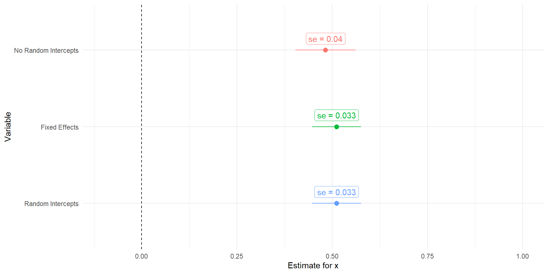
Note that the underlying data generating process has a different intercept based on our grouping variable
When we don’t account for this, the uncertainty in our regression coefficients increases dramatically
Depending on the severity of the problem, this can also result in bias being introduced in our regression coefficient

Random Intercepts

Code

tidy(fit2) %>% 
  mutate(model = 'No Random Intercepts') %>% 
  bind_rows(broom.mixed::tidy(fit_re) %>% 
              mutate(model = 'Random Intercepts'),
            tidy(fit3) %>% 
              mutate(model = 'Fixed Effects')) %>%
  mutate(model = factor(model,
                        levels = c('No Random Intercepts',
                                   'Fixed Effects',
                                   'Random Intercepts')),
         lower = estimate-1.96*std.error,
         upper = estimate+1.96*std.error) %>% 
  filter(term == 'x') %>%
  ggplot(aes(x = estimate, y = fct_rev(model), color = model))+
  geom_pointrange(aes(xmin = lower, xmax = upper))+
  geom_vline(aes(xintercept = 0), linetype = 2)+
  geom_label(aes(label = paste('se = ', round(std.error, 3),
                               sep = '')),
             nudge_y = .15)+
  labs(x = 'Estimate for x', y = 'Variable', color = 'Model')+
  xlim(-.1,1)+
  theme_minimal()+
  theme(legend.position = 'none')

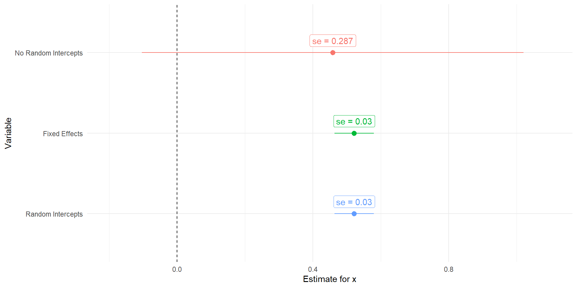
With more variation in the intercepts

The more different our intercepts are, the worse our uncertainty will get without the random intercepts

Code

set.seed(117)
#setting up our problem
##redrawing x
x <- rnorm(1000)

#setting up our grouping variable
groups <- c('g1','g2','g3','g4')
group <- sample(groups, size = 1000, replace = TRUE)

# Create group-specific intercepts (random intercepts)
group_intercepts <- rnorm(length(groups), mean = 0, sd = 10)
names(group_intercepts) <- groups

tibble(x     = x,
       group = group) %>% 
  group_by(group) %>% 
  mutate(group_int = group_intercepts[group],
    y = 1 + group_int + 0.5 * x + rnorm(n(), sd = 1)) -> reg_dat

#fitting our random intercepts model
fit_re <- lmer(y~x+(1|group), data = reg_dat)

#refitting a standard regression model
fit2 <- lm(y~x, data = reg_dat)

#including fixed effects instead
fit3 <- lm(y~x+group, data = reg_dat)

tidy(fit2) %>% 
  mutate(model = 'No Random Intercepts') %>% 
  bind_rows(broom.mixed::tidy(fit_re) %>% 
              mutate(model = 'Random Intercepts'),
            tidy(fit3) %>% 
              mutate(model = 'Fixed Effects')) %>%
  mutate(model = factor(model,
                        levels = c('No Random Intercepts',
                                   'Fixed Effects',
                                   'Random Intercepts')),
         lower = estimate-1.96*std.error,
         upper = estimate+1.96*std.error) %>% 
  filter(term == 'x') %>%
  ggplot(aes(x = estimate, y = fct_rev(model), color = model))+
  geom_pointrange(aes(xmin = lower, xmax = upper))+
  geom_vline(aes(xintercept = 0), linetype = 2)+
  geom_label(aes(label = paste('se = ', round(std.error, 3),
                               sep = '')),
             nudge_y = .15)+
  labs(x = 'Estimate for x', y = 'Variable', color = 'Model')+
  xlim(-.2,1.1)+
  theme_minimal()+
  theme(legend.position = 'none')